Closed-Loop Mixed-Signal Motor Speed Controller
Closed-loop speed regulation built from optical sensing, discrete timing logic, an 8-bit measurement path, analog feedback, and transistor motor drive.
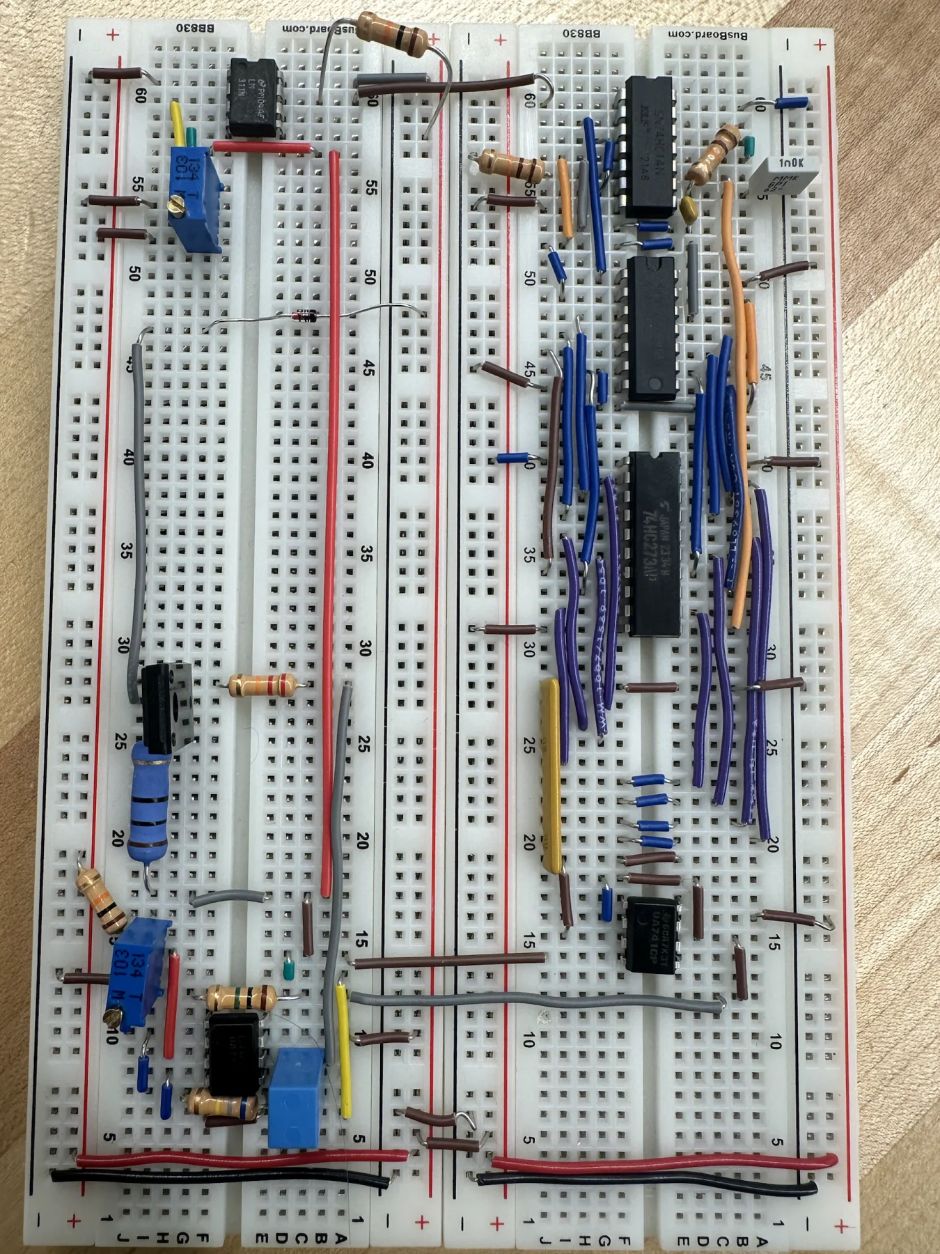
I implemented and tested a course-specified mixed-signal controller that measured a DC motor's shaft speed, held the result as an 8-bit value, converted it back to an analog feedback voltage, and adjusted the motor drive toward a potentiometer setpoint—without using a microcontroller.
Individual lab project · My work: breadboard implementation, subsystem validation, circuit analysis, instrumentation, integration, measurement-driven modifications, and fault isolation.
- Optical feedback
- 10 pulses / rev
- Measurement window
- 0.2 s
- Speed representation
- 8-bit
- Estimated test span
- 1200–3300 RPM
Build the feedback loop from first principles
The challenge was to close a motor-speed feedback loop using a chain of analog and digital building blocks. A potentiometer defined the target speed, while an optical sensor and slotted disk converted rotation into pulses that the circuit could measure.
The architecture was supplied for the final lab; the engineering work was in turning it into a functioning physical system, proving each stage with measurements, and separating wiring, instrumentation, control, power, and motor faults during integration.
No firmware abstraction
Timing, counting, memory, conversion, and feedback were all visible as voltages or digital states on the breadboard.
Mixed-signal boundaries
Sensor pulses had to become reliable logic, then an 8-bit result had to become a stable analog feedback voltage.
Real electromechanical load
The motor introduced current demand, component variation, noise, and failure modes that isolated signal tests did not reveal.
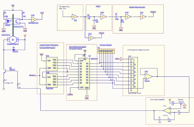
A loop across analog and digital domains
The control loop deliberately crosses the analog–digital boundary twice: rotation becomes pulses for counting, then the latched count becomes an analog voltage for comparison with the setpoint.
Ten optical pulses per shaft revolution encoded speed as a pulse frequency.
A 5 Hz timing chain latched the count every 0.2 s, then reset the counter for the next window.
The DAC voltage represented measured speed; the error amplifier compared it with the user-set target and drove the BJT stage.
The loop closes physically through the motor: drive changes shaft speed, which changes the optical pulse rate and therefore the next feedback measurement.
Latch first. Reset second.
The speed measurement only works if the previous count is saved before the counter is cleared. I used a delayed reset path so the register captured a stable value first, followed by a narrow reset pulse for the next measurement window.
- 01
Count
Accumulate optical pulses during the 0.2 s window.
- 02
Latch
Clock the 8-bit D register to preserve the measured count.
- 03
Delay
Use the RC and Schmitt-trigger path to separate latch and reset edges.
- 04
Reset
Clear the counter and begin the next independent measurement.
- Calculated RC delay
- 11 ± 1 µs
- Measured delay
- 12 ± 3 µs
- 50 Hz input over 0.2 s
- 10 counts
The calculated and measured delay intervals overlapped. A separate 50 Hz bench input produced a stored count of 10 in each 0.2 s window, confirming the counter, register, and timing relationship before motor integration.
Turning a digital count into feedback voltage
The latched binary count had to become an analog feedback level before it could be compared with the potentiometer setpoint. An 8-bit R–2R ladder performed the conversion and a voltage follower prevented the next stage from loading the ladder.
Vfeedback = (count / 255) × 5 V A known digital input produced the expected analog output
With a stored count of 10, the ideal DAC output is approximately 196 mV. I measured about 200 mV and confirmed that the buffer output matched the ladder output, providing an end-to-end check of the digital-to-analog bridge.
- Test count
- 10
- Calculated
- 196 mV
- Observed
- ≈ 200 mV
Making proportional and integral action visible
The error amplifier combined proportional and integral action. The proportional path responded immediately to a speed error, while the capacitor accumulated persistent error so the drive could continue correcting toward the setpoint.
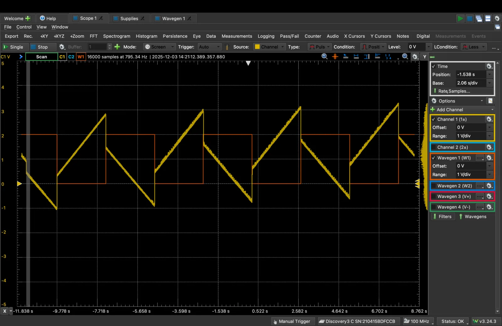
Vout = Vset + (1/RC)∫(Vset − Vfeedback)dt + (R7/R6)(Vset − Vfeedback) I tested the stage around a 1 V setpoint using a 1 Hz square-wave input that alternated between 0 V and 2 V. The output showed the expected immediate steps and linear ramps, making the proportional and integral contributions visible on the oscilloscope.
The waveform gradually drifted into the positive rail. I attributed that behavior to small DC mismatch being continually integrated. Rather than treating the clipped waveform as a clean pass, I documented the limitation and used the pre-saturation region to validate the intended response.
Debugging the interfaces between working blocks
The most valuable part of the project was learning to localize faults in a long mixed-signal chain. I stopped treating the controller as one circuit and verified boundaries one at a time with the oscilloscope, logic analyzer, and controlled test inputs.
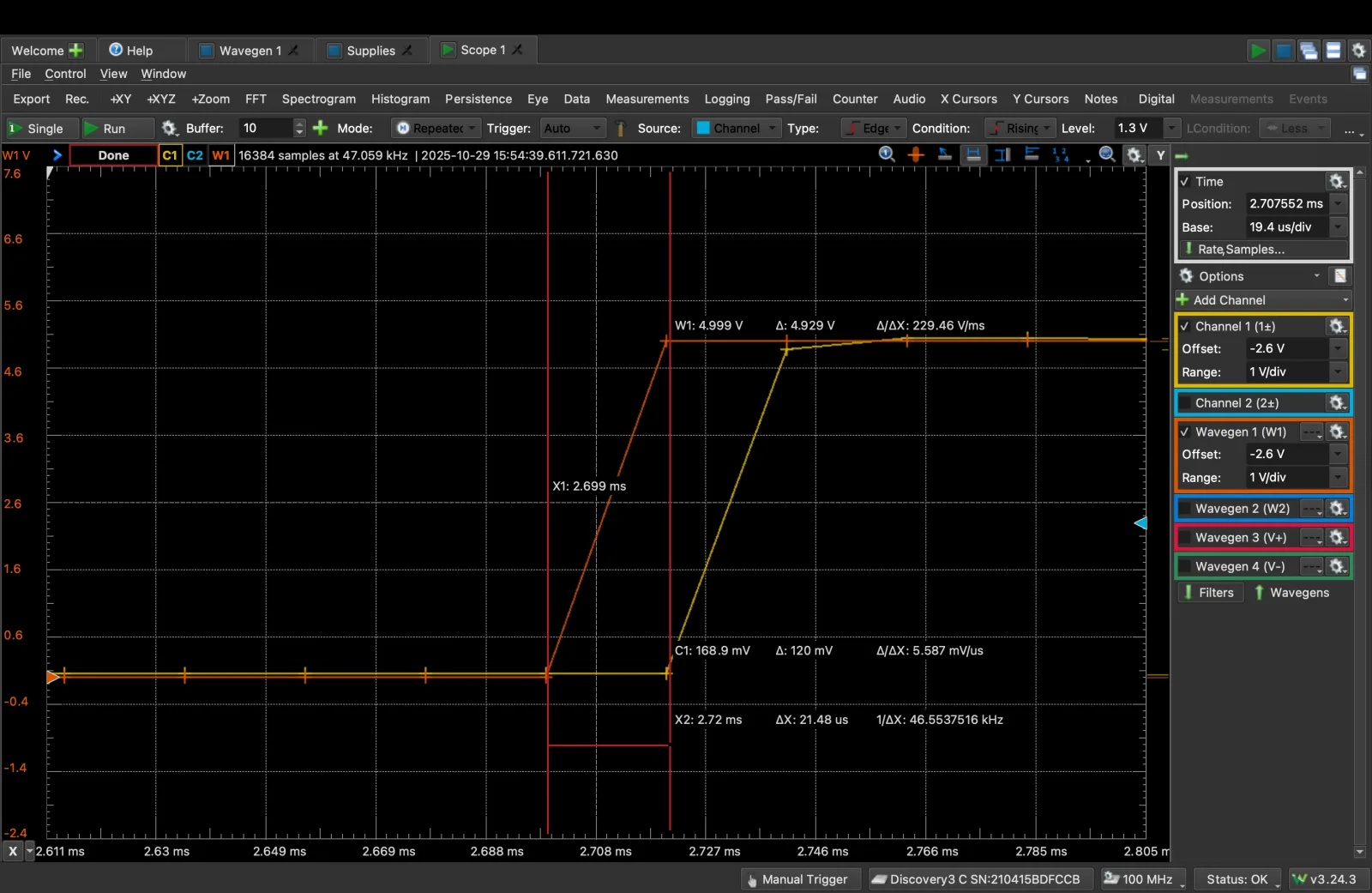
An invisible reset pulse
- Symptom
- The reset generator appeared to produce no output.
- Test
- I reviewed the expected RC timescale and changed the oscilloscope time base instead of immediately rewiring the circuit.
- Resolution
- The pulse was present but much narrower than the original viewing window.
Random latched values
- Symptom
- The register output fluctuated instead of holding the expected count.
- Test
- I probed the counter outputs, then the register inputs, and compared the two sides of their interconnect.
- Resolution
- The measurements isolated a wiring error between the counter and register.
A sensor pulse below threshold
- Symptom
- The motor sensor signal did not reliably toggle the Schmitt-trigger input.
- Test
- I scoped the sensor waveform and found that its low level did not cross the inverter threshold.
- Resolution
- I tested a comparator near 2.6 V and added the required pull-up for its open-collector output; the final replacement motor produced a usable signal without that extra stage.
Every block passed, but the loop failed
- Symptom
- Timing, counting, conversion, and error amplification worked independently, yet the integrated system did not regulate speed.
- Test
- I repeated subsystem tests, verified the powered instrument could supply the motor current, then substituted a known-good motor.
- Resolution
- The controller ran and followed the setpoint with the alternate motor, identifying the original motor as the system-level fault.
Setpoint, count, and estimated speed
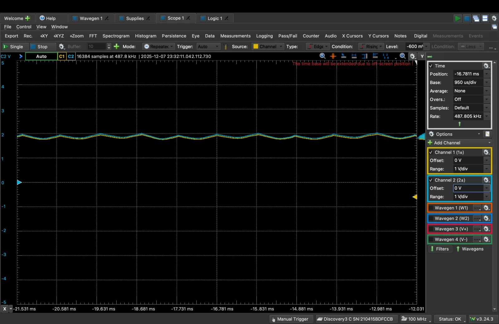
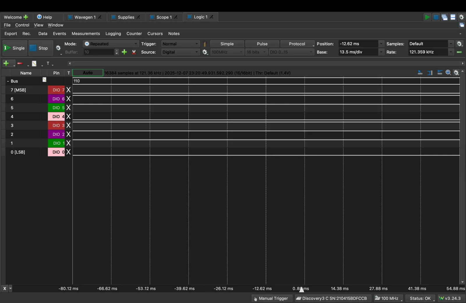
With the replacement motor, increasing the potentiometer setpoint increased the latched count and the DAC feedback voltage followed the setpoint. Using ten sensor pulses per revolution and a 0.2 s window, each count corresponded to 30 RPM.
Estimated speed = count × 5 windows/s × 60 s/min ÷ 10 pulses/rev = count × 30 RPM
| Setpoint | Latched count | Estimated speed |
|---|---|---|
| 0.7 V | 40 | 1200 RPM |
| 0.9 V | 50 | 1500 RPM |
| 1.1 V | 60 | 1800 RPM |
| 1.3 V | 70 | 2100 RPM |
| 1.5 V | 80 | 2400 RPM |
| 1.7 V | 90 | 2700 RPM |
| 1.9 V | 100 | 3000 RPM |
| 2.1 V | 110 | 3300 RPM |
The reported RPM values are calculated from the optical count rather than verified with an independent tachometer. Around a count of 110, the system stopped recovering cleanly when the setpoint was reduced, so I treat 3300 RPM as the observed edge of this prototype's useful range—not a guaranteed closed-loop specification.
What this project changed in my approach
Validate interfaces, not only blocks
A counter and register can both work independently while the wiring between them still fails. Boundary measurements made that distinction clear.
Measurement settings are part of the experiment
A signal can appear absent when the time base, trigger, threshold, or probe point does not match the phenomenon being tested.
Substitution is a legitimate diagnostic tool
Replacing the motor with a known-good unit narrowed a system-wide failure faster than continuing to rework already-validated control blocks.
Document the edge of validity
The high-speed recovery problem and integrator drift are part of the engineering result because they define where the prototype still needs refinement.